When I was in the market for an EV, one of the things I wondered about was how far I would be able to go outside the city before I had to charge it. Having a number for the range isn’t enough to know offhand whether I’d be able to reach a particular destination.

So I wanted to make the range more obvious in my EV guide by visualising vehicle range on a map.

The trivial solution is to use range as a radius and show a circle:

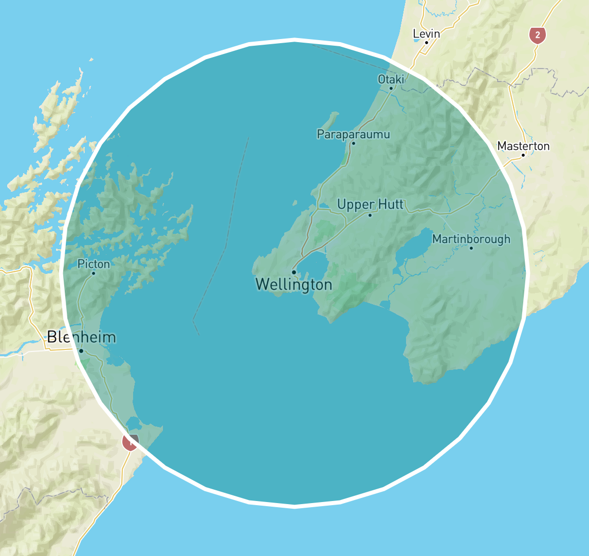
But of course, that’s going to be massively inaccurate because road distance isn’t at all the same as straight line distance.

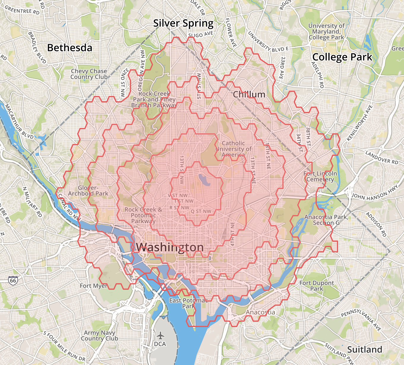
Instead, I needed to display a contour for a given distance when travelling by road. This contour is called an isodistance. Here is an example showing several isodistance contours from the Mapbox blog:

I determined that I would use a combination of PostGIS and Mapbox to generate the contours, and display them on a Mapbox map.

The basic approach is as follows:

• Generate a point grid around a given centre point
• For each point of the grid, calculate the travel distance using the Mapbox Directions API, which provides the road travel distance between given positions
• Discard all points which are further than the desired distance
• Calculate the convex hull of the remaining points - this is the isodistance contour.

With some experiments, I found out that the Mapbox Directions API considers some positions at sea to be reachable:

I know that Teslas can float, but surely not this far! Some of this may be because of ferry routes, but there are no ferry routes going northwards, for example. I thought it would be much better to have the isodistances limited to land. That meant I needed to exclude the points in the grid which are not on land from consideration.

So there were two tasks for me to complete with the help of PostgreSQL and PostGIS:

• Generate a point grid in the relevant area
• Discard points which are not on land

Generating a point grid

Once inside a freshly created database in psql, I needed to install the PostGIS functions:

create extension postgis;
create extension postgis_topology;

The first approach I tried (described on Stack Exchange) consists of taking a box (eg the bounding box of some polygon) and using generate_series to produce the coordinates of the points.

This approach requires producing the coordinates of the bounding box. There was a problem with that: since I was visualising EV range, I wanted to work with kilometres, and PostGIS doesn’t provide an easy way to specify, say, a radius for a circle of geometry type in kilometres.

This led me to look at the geography type, but I struck another problem. Being centred in New Zealand, my bounding polygon happened to cross the international dateline, and PostGIS was unable to produce meaningful results.

Finally, I found the st_project function, which allowed me to move a point by providing a distance and azimuth.

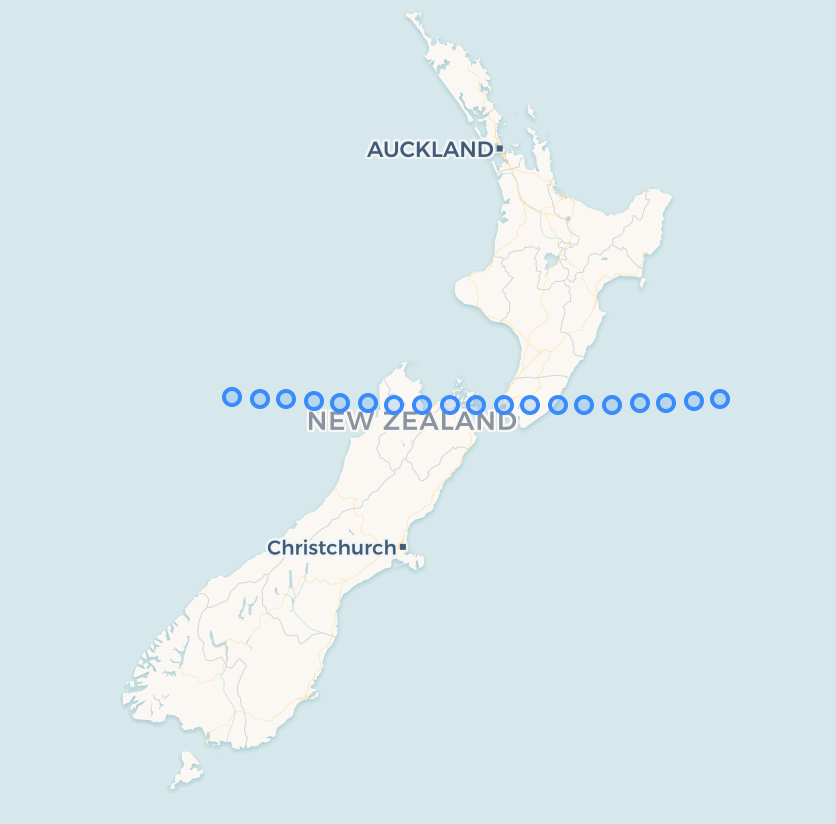
I started by generating a line of points 50km apart:

select st_project(st_setSrid(st_point(174.8431, -41.2581), 4326)::geography, s.a * 50000, pi() / 2) as pt
from generate_series(-10, 10, 1) as s(a)

A couple of asides:

• The 50km gap between points isn’t actually practical – such a grid is too sparse to produce useful isodistance contours. In actual fact, I used 10km, but that’s hard to visualise as the points merge into a single blob of colour.
• The screenshots in this post are from pgAdmin 4 which is able to visualise result sets of geometry and geography types. It’s incredibly useful.

Then, I expanded it into a grid with another application of generate_series:

with row as (
    select st_project(st_setSrid(st_point(174.8431, -41.2581), 4326)::geography, 
        s.a * 50000, pi() / 2) as pt
    from generate_series(-10, 10, 1) as s(a)
)
select st_project(pt, s.a * 50000, 0) as projected_pt
from row, generate_series(-10, 10, 1) as s(a)

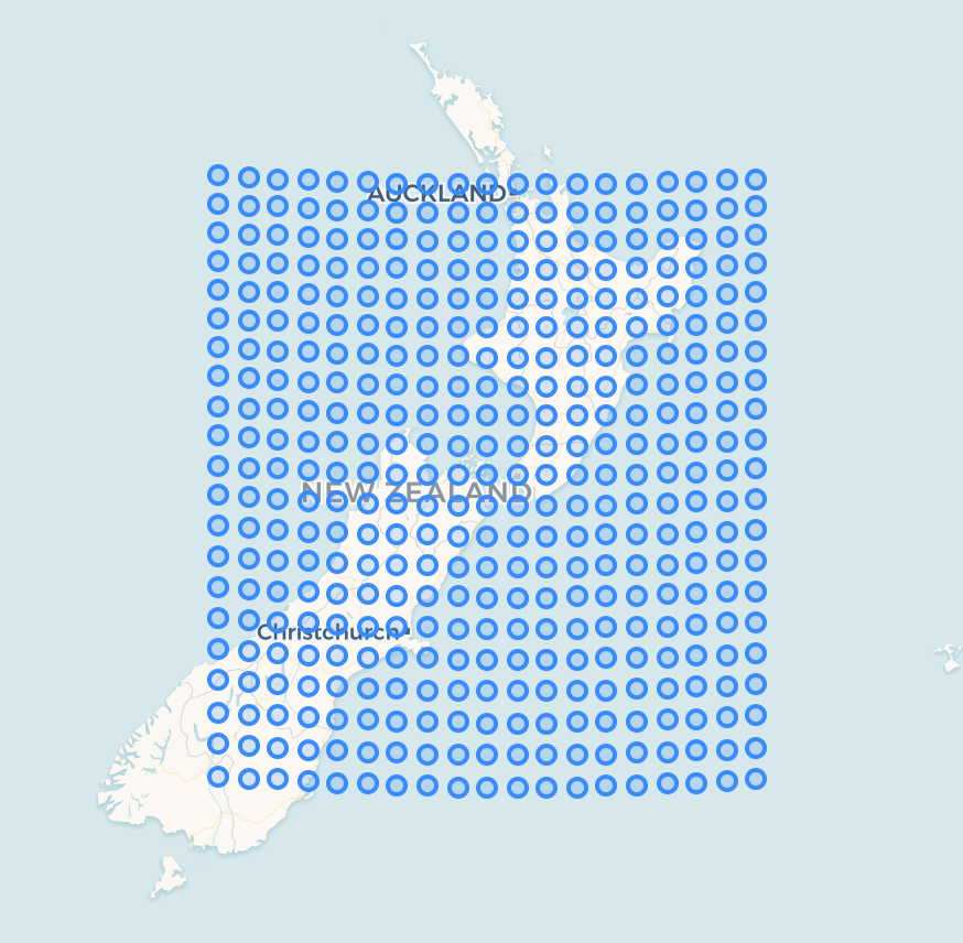
The fact that the grid doesn’t look square is a display artifact. Some points are across the dateline so they aren’t shown (they appear at the other end of the map instead).

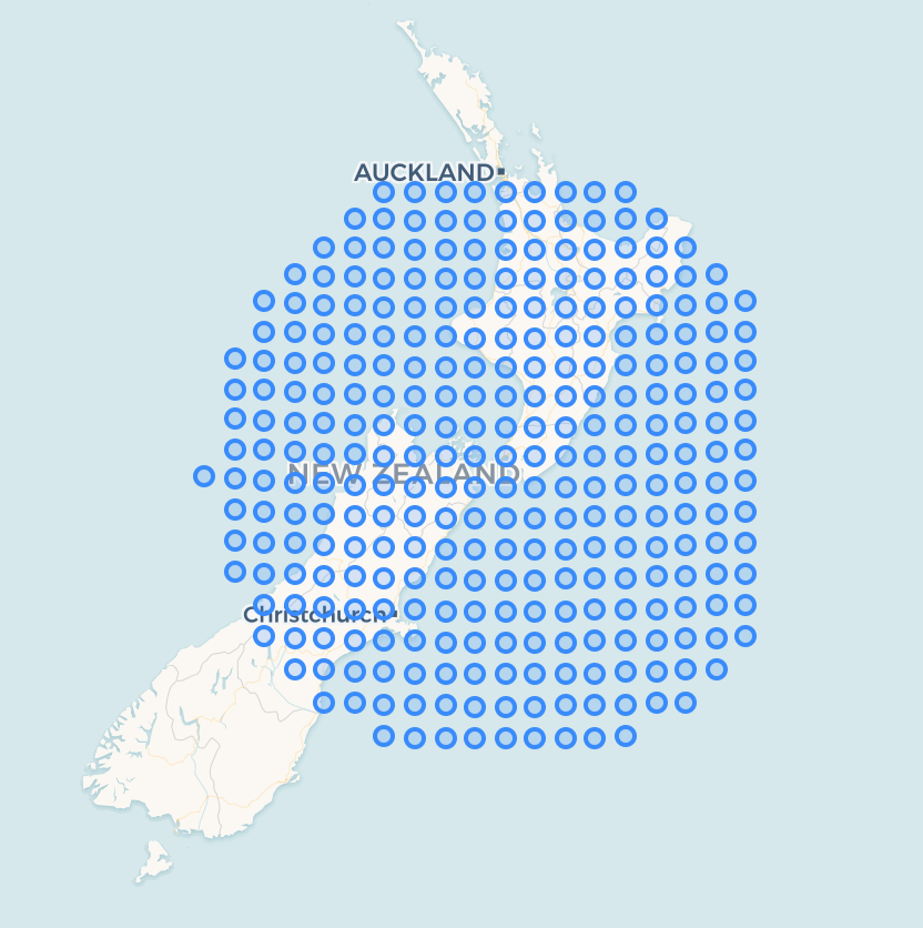
An obvious constraint is that points can’t be more than a certain straight line distance from the origin, so I added that in to discard points outside the 500km radius:

with row as (
    select st_project(st_setSrid(st_point(174.8431, -41.2581), 4326)::geography,
        s.a * 50000, pi() / 2) as pt
    from generate_series(-10, 10, 1) as s(a)
)
select st_project(pt, s.a * 50000, 0) as projected_pt
from row, generate_series(-10, 10, 1) as s(a)
where st_distance(st_setSrid(st_point(174.8431, -41.2581), 4326)::geography
    , st_project(pt, s.a * 50000, 0)) < 500000

And that was it – I had a point grid! On to the second task then.

Discarding positions at sea

The next step was to remove the points which are not on land from consideration.

New Zealand land contours are available from Land Information New Zealand in the form of a 21MB KML file containing polygons comprised of several hundred thousand points. To import this data into PostgreSQL, I knew I could use the ogr2ogr tool which is part of the GDAL package (brew install gdal on macOS):

$ ogr2ogr -f "PostgreSQL" PG:"host=localhost user=alex dbname=isodist password=" nz-coastlines-and-islands-polygons-topo-150k.kml

This produced a table with the geometries imported as binary strings:

isodist=# \dt
                             List of relations
┌────────┬─────────────────────────────────────────────────┬───────┬───────┐
│ Schema │                      Name                       │ Type  │ Owner │
├────────┼─────────────────────────────────────────────────┼───────┼───────┤
│ public │ nz coastlines and islands polygons (topo 1:50k) │ table │ alex  │
└────────┴─────────────────────────────────────────────────┴───────┴───────┘

isodist=# \d public."nz coastlines and islands polygons (topo 1:50k)"

┌──────────────┬───────────────────┬───────────┬──────────┬
│    Column    │       Type        │ Collation │ Nullable │                               
├──────────────┼───────────────────┼───────────┼──────────┼
│ ogc_fid      │ integer           │           │ not null │ 
│ wkb_geometry │ bytea             │           │          │
│ name         │ character varying │           │          │
│ description  │ character varying │           │          │
└──────────────┴───────────────────┴───────────┴──────────┴

After renaming the table to coastlines, I could run the following query to see which geometries contain a given point (say (175.9065, -38.7797)):

with geoms as (
    select st_setsrid(encode(wkb_geometry, 'hex'), 4326) as g from coastlines
) 
select st_geometrytype(g)
    , st_npoints(g)
    , st_contains(g, st_setsrid(st_point(175.9065, -38.7797), 4326)) 
from geoms 
order by 2 desc;

The geometries had to be encoded into a textual representation (in the geoms CTE) to be passed to PostGIS functions. st_contains is a PostGIS function which returns true if the first geometry contains the second.

Finally, I could combine the point grid query with a where clause to discard positions at sea:

with geoms as (
    select st_setsrid(encode(wkb_geometry, 'hex'), 4326) as g from coastlines
) 
, row as (
    select st_project(st_setSrid(st_point(174.8431, -41.2581), 4326)::geography, s.a * 50000, pi() / 2) as pt
    from generate_series(-10, 10, 1) as s(a)
)
select st_project(pt, s.a * 50000, 0) as projected_pt
from row, generate_series(-10, 10, 1) as s(a)
where st_distance(st_setSrid(st_point(174.8431, -41.2581), 4326)::geography, st_project(pt, s.a * 50000, 0)) < 500000
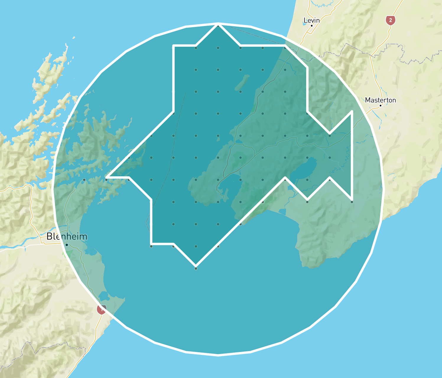
    and exists(select 1 from geoms where st_nPoints(g) > 1000 and st_contains(g, st_project(pt, s.a * 50000, 0)::geometry))

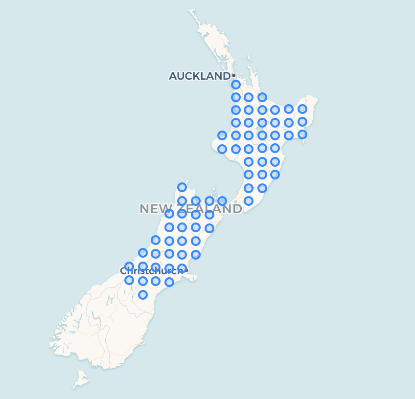
I only applied the st_contains check to land contours made up of over 1000 points (st_nPoints(g) > 1000) because it wasn’t necessary for me to check exhaustively against all the little islands and the like.

This produced the following result:

At this point, I could write out the result set as a JSON array of coordinates with the help of PostgreSQL JSON functions to use it with the Mapbox Directions API:

with geoms as (
    select st_setsrid(encode(wkb_geometry, 'hex'), 4326) as g from coastlines
) 
, row as (
    select st_project(st_setSrid(st_point(174.8431, -41.2581), 4326)::geography, s.a * 50000, pi() / 2) as pt
    from generate_series(-10, 10, 1) as s(a)
)
, grid as (
    select st_project(pt, s.a * 50000, 0)::geometry as projected_pt
    from row, generate_series(-10, 10, 1) as s(a)
    where st_distance(st_setSrid(st_point(174.8431, -41.2581), 4326)::geography, st_project(pt, s.a * 50000, 0)) < 500000
        and exists(select 1 from geoms where st_nPoints(g) > 1000 and st_contains(g, st_project(pt, s.a * 50000, 0)::geometry))
)
, coords as (
    select st_x(projected_pt) as lon, st_y(projected_pt) as lat 
    from grid
)
select json_agg(row_to_json(coords)) from coords

Conclusion

There are a couple of points to make in conclusion:

• PostgreSQL and PostGIS provide a powerful set of tools which allowed me to achieve my goal of producing a land-constrained point grid with a single, surprisingly short query.
• Having the land contours available as a public dataset makes it possible to do useful things with geographical data in side projects like mine, citizen science and the like.